Recommendation Systems Walkthrough - Build Content Based Recommenders
This Post Discusses different approaches for recommending movies based on the content of the movie and not just the user preferences.
We previously discussed how we built a recommender module based on user preferences, you may want to read about the story here. We used different similar movies to match the user preferences in movie taste.
In this post, we are going to make use of the content available in the movie like
- Movie Title
- Movie Summary
- Movie Description
- Movie Category
- Movie Director / Actor / Casting Team

Content based filtering make recommendations by using items metadata such as genres, title, description actors, director … etc.
So we can say if a user liked a particular item he also may like similar items to it.
A lot of meta metadata about movies can be used to build movie recommendations based on the content. We can make use of the movie title in which we can say that similar movies may have similar titles. Also, the movie description may be informative about how we represent similarities between movies.
What about the Cast team and directors? I would like to watch movies by the same director again.
Architecture Overview
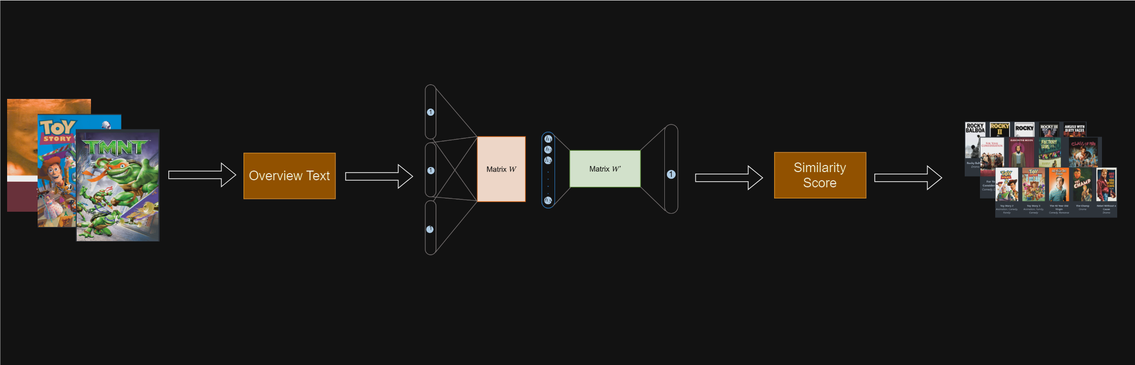
Embeddings
Embedding models have revolutionized how language is being used in the NLP era. I am not going to focus on how embeddings models is working here rather than focus on its usability for vectorizing text to use in suggestion engine pipeline.
Why embeddings and not simpler representation like TFIDF ?
Embeddings models in information retrieval systems has many powerful preferences over the traditional TF-IDF method, One of the most reasons is:
Word2Vec Creates dense vector representations where words with similar meanings are positioned closer together in the vector space. For example, “king” and “queen” will be closer in the vector space, capturing their semantic similarity.
TF-IDF Treats words as independent features and does not capture any semantic relationship between them. It only considers the frequency and distribution of words, so “king” and “queen” would be treated as entirely separate features.
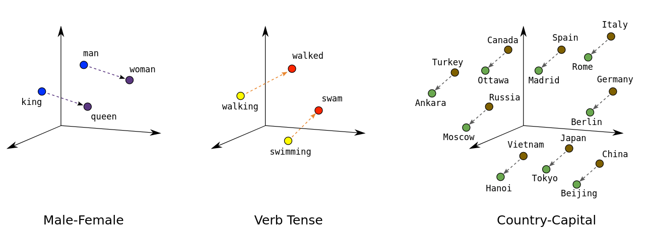
Word2Vec Reduces the dimensionality of the representation by embedding words into a continuous vector space of typically a few hundred dimensions (e.g., 100-300 dimensions). This helps in reducing computational complexity and memory usage.
TF-IDF Results in a sparse matrix where the number of dimensions equals the size of the vocabulary. For large corpora, this can lead to very high-dimensional data, which can be computationally expensive to process.
To read more about embeddings models and how it works behind the hood i will just leave this wonderful articles
So in summary, We are going to use Word2vec Embeddings model to represent textual content of a movie and feed it to similarity scoring system in order to extract the most similar items.
Since we have a semantic representation of the textual content of the movies metadata, it is expected to have a good scoring system.
I trained Word2vec model using skip-gram architecture on vocabulary of size 544115 token and 10000 movies description from TMDB database using skip-gram GPU.
There is a specific kind of confidence that comes from watching your first recommendation engine return results. You feed it The Dark Knight, and it returns Batman Begins and Inception. It works. You close the laptop satisfied. What you do not yet know is that you have built a system that will quietly collapse the moment it faces real data at real scale. This post is the story of that collapse — and the architectural journey required to fix it.
1. The “Weekend Project” Trap
The Seductive Simplicity of Word2Vec
The baseline architecture described in most introductory tutorials follows the same pattern: train (or load) a Word2Vec model, represent each movie by averaging the vectors of all tokens in its description, and then rank candidates by cosine similarity against a query movie’s averaged vector.
# Baseline Word2Vec token-averaging
def get_movie_vector(description: str, model: Word2Vec) -> np.ndarray:
    tokens = description.lower().split()
    vectors = [model.wv[t] for t in tokens if t in model.wv]
    return np.mean(vectors, axis=0) if vectors else np.zeros(model.vector_size)

def find_similar_baseline(query_title: str, df: pd.DataFrame, model: Word2Vec):
    query_vec = get_movie_vector(df.loc[query_title, "description"], model)
    scores = df["description"].apply(
        lambda d: cosine_similarity([query_vec], [get_movie_vector(d, model)])[0][0]
    )
    return scores.nlargest(10)
This is the “Hello World” of recommendation systems, and it deserves credit for being approachable. It introduces the right vocabulary — vectors, embeddings, semantic distance — and produces results that are directionally sensible.
But before diagnosing its failures, it is worth understanding exactly how this baseline learns its representations — because the architecture choice (Skip-gram vs CBOW) reveals precisely where the ceiling is.
Skip-gram vs CBOW: The Right Choice for the Wrong Reason
Word2Vec comes in two training architectures, and they are not interchangeable.
CBOW (Continuous Bag of Words) takes a window of surrounding context words and predicts the target word in the middle. Given [“A”, “man”, “_”, “a”, “bank”], CBOW predicts “robs”. It averages the context vectors before predicting, which makes it fast and stable on high-frequency vocabulary — but that averaging discards word order before training even begins.
Skip-gram inverts this: given a single target word “robs”, it predicts each of the surrounding context words individually. This is slower and computationally heavier, but it learns significantly richer representations for rare and domain-specific terms — exactly the kind of vocabulary that dominates a movie metadata corpus: director names, character names, genre-specific terminology, film titles.
CBOW:   [context window] ──── avg ────► predict target word
Skip-gram:  target word ──────────────► predict each context word
The TMDB-based baseline described in the walkthrough — trained on 10,000 movie descriptions with a ~544,000 token vocabulary — made the right call choosing Skip-gram. That vocabulary is sparse and domain-specific. CBOW would have underrepresented rare but semantically critical tokens like “Kubrickian”, “neo-noir”, or a director’s surname appearing only a handful of times.
So why is Skip-gram still insufficient?
Both CBOW and Skip-gram produce static embeddings. Every token receives one fixed vector, determined once during training and never updated based on context at inference time. The word “dark” in “dark comedy” gets the same vector as “dark” in “The Dark Knight.” The word “not” contributes its vector to the average — but averaging has no mechanism to encode negation. “A hero who is not what he seems” and “A hero who is exactly what he seems” produce nearly identical document vectors.
This is the ceiling that neither Skip-gram nor CBOW can escape: the averaging step that converts word vectors into a document representation is a lossy compression with no awareness of syntax, order, or cross-token dependencies. It is not a flaw in the training objective — it is a structural limit of the representation method.
Key Takeaway: Skip-gram was the correct architecture choice for a sparse, domain-specific vocabulary. But both Skip-gram and CBOW share the same fundamental limit: static, context-free token vectors that lose sentence structure the moment they are averaged.
But it has two structural flaws that are fatal in production.
Flaw 1 — Token Averaging Destroys Context
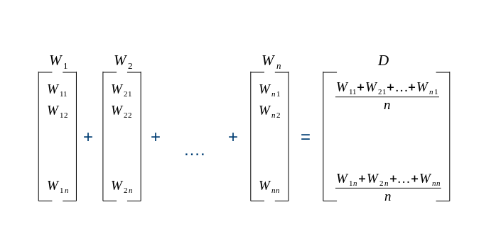
Word2Vec operates at the word level. Each token gets a fixed vector, and those vectors are averaged together to form a document representation. This means the sentence “A man who is not what he seems” produces the exact same vector regardless of word order, negation, or syntactic structure. The model has no concept of “not.”
More critically: Word2Vec is a static embedding. The word “dark” has one vector, whether it appears in “dark comedy” or “Dark Knight” or “after dark.” The contextual relationship between tokens is irretrievably lost in the averaging step.
The result is a representation that captures loose topic proximity but misses plot nuance, tone, and intent entirely.
Flaw 2 — Linear Search Does Not Scale
The find_similar_baseline function above computes cosine similarity against every item in the catalog, one at a time. At 1,000 movies this is invisible latency. At 100,000 movies — a realistic streaming catalog — you are performing 100,000 dot product operations per query. At 1,000,000 movies (Netflix scale), this is simply not deployable.
The time complexity is O(N) per query. Every item added to the catalog makes every future query slower by a fixed increment.
Key Takeaway: A system that works on a 1,000-item sample can be non-functional on production data. “It works on my dataset” is not a readiness signal — it is the beginning of the engineering problem.
2. Leveling Up: From Words to Sentences
The Context Problem
Consider these two movie descriptions:
- “A man robs a bank to fund his dying wife’s treatment.”
- “A man deposits his life savings in a bank near the river.”
A Word2Vec model averaging token vectors will place these descriptions relatively close together. Both contain “man,” “bank,” and financial connotations. The semantic distance between them, as far as token-averaging is concerned, is small.
A human reader understands these are describing entirely different dramatic situations. The word “bank” means something different in each sentence — and critically, the intent of the narrative is opposite.
This is the problem that Sentence Transformers (SBERT) were designed to solve.
How SBERT Works
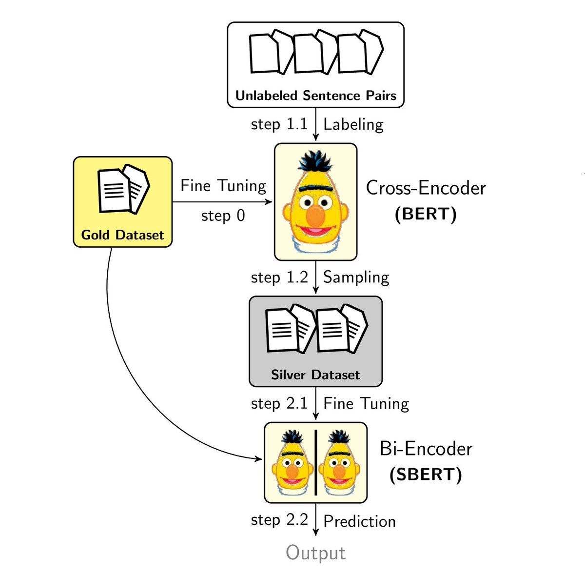
SBERT is built on top of a pre-trained transformer (typically BERT or RoBERTa) and fine-tuned using a Siamese network architecture on sentence-pair similarity tasks. The result is a model that produces a single fixed-size embedding for an entire sentence or paragraph, where that embedding encodes contextual meaning across the full input sequence.
Under the hood, the transformer’s multi-head self-attention mechanism allows every token in the input to attend to every other token before the final representation is computed. This is what gives SBERT its contextual awareness — “bank” near “river” activates different attention patterns than “bank” near “robbery.”
The final sentence vector is typically produced by mean pooling across all token states in the last transformer layer, then normalized to unit length for efficient cosine similarity computation.
Choosing the Right Model
For a production recommendation system, all-MiniLM-L6-v2 is the correct starting point. Here is why:
| Model | Embedding Dim | Speed (sentences/sec) | Semantic Quality |
all-MiniLM-L6-v2 |
384 | ~14,000 | Strong |
all-mpnet-base-v2 |
768 | ~2,800 | Best-in-class |
| Word2Vec (custom) | 100–300 | ~50,000 | Weak (no context) |
all-MiniLM-L6-v2 offers 80% of mpnet’s quality at 5x the throughput. For a catalog of 100k movies that needs periodic re-indexing, that throughput gap is the difference between a 10-minute batch job and an 80-minute one.
The MovieEmbedder Class
# MovieEmbedder class
from sentence_transformers import SentenceTransformer
import numpy as np
from typing import List

class MovieEmbedder:
    """
    Wraps a Sentence-Transformer model and provides batch-efficient
    embedding generation for movie metadata strings.
    """
    def __init__(self, model_name: str = "all-MiniLM-L6-v2", batch_size: int = 64):
        self.model = SentenceTransformer(model_name)
        self.batch_size = batch_size
        self.embedding_dim = self.model.get_sentence_embedding_dimension()

    def embed(self, texts: List[str], show_progress: bool = True) -> np.ndarray:
        """
        Generate L2-normalized embeddings for a list of input strings.
        Uses batched inference to manage memory on large catalogs.

        Returns:
            np.ndarray of shape (len(texts), embedding_dim), float32
        """
        embeddings = self.model.encode(
            texts,
            batch_size=self.batch_size,
            show_progress_bar=show_progress,
            normalize_embeddings=True,   # Unit vectors → cosine sim = dot product
            convert_to_numpy=True
        )
        return embeddings.astype(np.float32)
Two implementation details are worth noting here:
normalize_embeddings=True— When vectors are unit-normalized, cosine similarity reduces to a simple dot product. FAISS (introduced in Section 4) can exploit this with itsIndexFlatIP(inner product) index, which is faster than computing full cosine similarity.batch_size=64— Loading all descriptions into GPU memory simultaneously will cause OOM errors on large catalogs. Batched encoding processes the corpus in chunks, keeping memory usage constant regardless of catalog size.
Key Takeaway: Sentence Transformers don’t just “do Word2Vec better” — they operate at a fundamentally different level of abstraction. A Word2Vec model understands tokens; an SBERT model understands meaning.
3. The Metadata Soup Strategy
Why Text Alone Under-Specifies a Movie
Imagine two films with nearly identical descriptions: both are “A lone protagonist battles a corrupt system to protect the ones they love.” One is a gritty Christopher Nolan crime thriller. The other is an animated family adventure.
The plot description is near-identical. The viewing experience is not. A recommendation engine operating only on description text will treat these films as twins.
This is not an edge case — it is a structural failure mode. Text descriptions encode narrative events. They do not reliably encode tone, genre conventions, directorial style, or audience intent. A horror film and a thriller can share nearly identical plot summaries. A critically acclaimed arthouse drama and a mainstream blockbuster can describe the same story beats in the same words. The description is a partial signal, and building a recommendation system on partial signals produces partial results.
A production system needs to encode what type of film this is, not just what happens in it.
There are two distinct strategies for doing this, and they make different trade-offs. Understanding both — and when to use each — is the engineering decision at the core of feature enrichment.
Strategy 1 — The Metadata Soup (Early Fusion)
The soup approach constructs a single enriched string per movie by concatenating all relevant metadata fields before embedding. The transformer encodes this combined string as one unified input sequence.
"Genre: Action Sci-Fi Action Sci-Fi | Director: Christopher Nolan |
 Cast: Leonardo DiCaprio Joseph Gordon-Levitt |
 Description: A thief who steals corporate secrets through dream-sharing
 technology is given the inverse task of planting an idea."
The key implementation detail is token repetition as a weight proxy. Because the transformer allocates attention across all tokens in the sequence, repeating a field increases the proportion of the sequence that field occupies — and therefore increases its influence on the final embedding. Repeating "Action Sci-Fi" twice is a blunt approximation of assigning that field a 2x weight.
# build_metadata_soup() with structured prefix formatting
def build_metadata_soup(row: pd.Series) -> str:
    """
    Constructs a weighted metadata string for a single movie record.

    Design decisions:
      - Field prefixes ("Genre:", "Director:") help the transformer
        contextualise each token cluster as a distinct semantic category.
      - Description is placed last so genre/director tokens appear early
        in the attention window, improving their influence on pooling.
      - Genre repeated 2x: strongest categorical signal.
      - Director repeated 1x: stylistic signal; sparse but high-value.
      - Cast limited to top 3: diminishing returns beyond lead actors.

    Args:
        row: A pandas Series representing one movie record.

    Returns:
        A single concatenated string ready for SBERT embedding.
    """
    genre     = str(row.get("genre", "")).strip()
    director  = str(row.get("director", "")).strip()
    cast      = ", ".join(str(row.get("cast", "")).split(",")[:3]).strip()
    desc      = str(row.get("description", "")).strip()

    parts = []
    if genre:    parts.append(f"Genre: {genre} {genre}")       # 2x weight
    if director: parts.append(f"Director: {director}")         # 1x weight
    if cast:     parts.append(f"Cast: {cast}")                 # 1x weight
    if desc:     parts.append(f"Description: {desc}")          # full weight

    return " | ".join(parts).lower().strip()
When the soup works well:
- When description and metadata are coherently related (a horror film with horror-coded descriptions)
- When you want a single FAISS index and a simple query path
- When catalog size makes maintaining multiple indexes expensive
When the soup breaks down:
- When a comedy has a dark, serious description (the dark words problem in your reference above)
- When a director has a wildly varied filmography and their name alone is a weak signal
- When categorical fields are inconsistently populated across your dataset
The soup is fast, simple, and good enough for most catalogs. But it makes one irreversible decision: once you concatenate everything into one string and embed it, you cannot adjust the relative influence of genre vs. description at query time without re-embedding the entire catalog.
Strategy 2 — Weighted Feature Vectors (Late Fusion)
Late fusion takes a different approach: embed each field independently, producing a separate similarity score per field, then combine those scores at query time using a weighted formula.
\[\text{Final Score} = w_1 \cdot \text{Sim}_{\text{desc}}(q, d) + w_2 \cdot \text{Sim}_{\text{genre}}(q, d) + w_3 \cdot \text{Sim}_{\text{director}}(q, d)\]Where each $\text{Sim}$ term is the cosine similarity between the query movie’s field embedding and the candidate movie’s field embedding, and the weights $w_1 + w_2 + w_3 = 1.0$.
This means maintaining three separate embedding vectors per movie — one for description, one for genre, one for director/cast — and computing three similarity scores at retrieval time before combining them.
# Late fusion scoring with per-field similarity matrices
import numpy as np
from dataclasses import dataclass
from typing import Dict

@dataclass
class MovieFeatureVectors:
    """Stores separate L2-normalized embeddings per feature field."""
    desc_vec:     np.ndarray   # shape: (embedding_dim,)
    genre_vec:    np.ndarray
    director_vec: np.ndarray

#  Weight configuration (tune via offline evaluation)
FIELD_WEIGHTS = {
    "desc":     0.60,   # Plot semantics: highest signal for content similarity
    "genre":    0.25,   # Categorical match: strong but coarse
    "director": 0.15,   # Stylistic signal: sparse but highly discriminative
}

def late_fusion_score(
    query: MovieFeatureVectors,
    candidate: MovieFeatureVectors,
    weights: Dict[str, float] = FIELD_WEIGHTS
) -> float:
    """
    Compute a weighted similarity score between two movies
    using per-field dot products (valid for L2-normalized vectors).

    Returns:
        Scalar score in range [-1.0, 1.0]. Higher = more similar.
    """
    desc_sim     = float(query.desc_vec     @ candidate.desc_vec)
    genre_sim    = float(query.genre_vec    @ candidate.genre_vec)
    director_sim = float(query.director_vec @ candidate.director_vec)

    return (
        weights["desc"]     * desc_sim +
        weights["genre"]    * genre_sim +
        weights["director"] * director_sim
    )
The critical advantage of late fusion is that the weights $w_1, w_2, w_3$ are query-time parameters. You can change them without re-embedding anything. This unlocks a class of personalisation that early fusion cannot support:
- A user who consistently watches films by the same director → increase $w_3$
- A user who jumps between genres → decrease $w_2$
- A query where description quality is low (missing or very short) → reduce $w_1$ and compensate with $w_2$
This is also how you solve the dark words problem explicitly. If a comedy has a grim, serious description, its desc_sim against another comedy may be low — but its genre_sim will be high. Late fusion lets genre catch what description misses.
# Dynamic weight adjustment by query context
def get_adaptive_weights(query_row: pd.Series) -> Dict[str, float]:
    """
    Adjust field weights based on query movie characteristics.
    Returns normalised weights that sum to 1.0.
    """
    desc_len = len(str(query_row.get("description", "")).split())
    weights = FIELD_WEIGHTS.copy()

    # Short/missing descriptions are unreliable — down-weight them
    if desc_len < 15:
        weights["desc"]  = 0.30
        weights["genre"] = 0.45

    # Normalize so weights always sum to 1.0
    total = sum(weights.values())
    return {k: v / total for k, v in weights.items()}
Choosing Between Strategies: A Decision Framework
| Criterion | Metadata Soup (Early Fusion) | Weighted Vectors (Late Fusion) |
| Implementation complexity | Low — one embedding per movie | High — N embeddings per movie |
| Index infrastructure | Single FAISS index | One FAISS index per field, or score at retrieval |
| Weight adjustment | Requires full re-embedding | Query-time parameter, no re-embedding |
| Handles sparse fields | Poorly — missing fields leave gaps | Gracefully — zero-weight missing fields |
| Handles description/genre mismatch | Poorly — blended signal averages out | Well — genre score compensates |
| Best for | Catalog ≤ 500k, stable metadata schema | Catalog with variable field quality, personalisation needed |
In practice, most production systems start with a soup approach and migrate to late fusion when they hit the weight-adjustment limitation — typically when a product team asks “can we surface more films by this director?” and the engineering answer is “only if we re-embed the entire catalog.”
Signal Value by Field: What Each Metadata Type Actually Encodes
Not all fields carry equal information. Understanding what each field actually signals prevents over-engineering low-value metadata while under-weighting high-value fields.
| Field | Signal Type | Sparsity | Recommended Weight Range |
| Description | Plot semantics, tone, narrative arc | Low (usually populated) | 0.50 – 0.65 |
| Genre | Audience expectation, content conventions | Low | 0.20 – 0.30 |
| Director | Visual style, pacing, thematic preoccupations | Medium (indie films often missing) | 0.10 – 0.20 |
| Lead Cast | Star power, performance style, fan affinity | Medium | 0.05 – 0.15 |
| Keywords / Tags | Mood, setting, subgenre nuance | High (inconsistently populated) | 0.05 – 0.10 |
| Runtime | Audience commitment signal | Low | Context-dependent only |
Keywords deserve a specific note. When populated consistently, they are the highest-precision field in the dataset — a tag like “psychological thriller” or “found footage” is more discriminative than any description sentence. But keyword coverage in TMDB and similar databases is uneven. Treat keywords as a high-upside, high-risk field: include them when present, do not penalise their absence.
Key Takeaway: The choice between metadata soup and weighted late fusion is not a question of correctness — both produce valid recommendations. It is a question of what you need to change at runtime. If your weights are fixed, use the soup. If you need to adjust feature influence per query, per user, or per business rule, late fusion is the only architecture that supports it without re-embedding.
4. Infrastructure Matters: The Vector Store
The Library Analogy
Imagine a library with one million books. You need to find the 10 books most similar to the one you are holding.
The baseline approach is equivalent to walking through every aisle, pulling out every book, and comparing it to yours — one by one. This is O(N) search. At a million books, it is not a library; it is a warehouse with no index.
A vector database with an HNSW index is the equivalent of the library’s card catalog system — but instead of alphabetical sorting, the catalog is organized by semantic neighborhood. Books on similar topics are clustered in adjacent sections. To find your 10 similar books, you navigate directly to the relevant section and compare only the books there. You might examine 50 books instead of 1,000,000.
This is the intuition behind Approximate Nearest Neighbor (ANN) search.
FAISS and the HNSW Index
FAISS (Facebook AI Similarity Search) is the industry-standard library for this operation. Its HNSW (Hierarchical Navigable Small World) index builds a multi-layer graph structure over the embedding space during index construction. Each node (movie) is connected to its nearest neighbors across multiple graph layers.
At query time, the search traverses this graph starting at the top (coarse) layer and descending to progressively finer layers, narrowing the candidate set at each step. The traversal is O(log N) — the number of comparisons grows logarithmically with catalog size, not linearly.
The two key construction parameters are:
| Parameter | What it Controls | Practical Range |
M |
Number of neighbors per node per layer. Higher = better recall, more memory. | 16–64 |
ef_construction |
Candidate pool size during index build. Higher = better index quality, slower build. | 100–400 |
The VectorStoreManager Class
import faiss
import numpy as np
import pickle
from pathlib import Path

class VectorStoreManager:
    """
    Manages a FAISS HNSW index: build, persist to disk, load, and query.
    Uses IndexHNSWFlat with inner-product metric (requires L2-normalized vectors).
    """
    def __init__(self, embedding_dim: int, M: int = 32, ef_construction: int = 200):
        self.embedding_dim = embedding_dim
        self.index = faiss.IndexHNSWFlat(embedding_dim, M, faiss.METRIC_INNER_PRODUCT)
        self.index.hnsw.efConstruction = ef_construction
        self.index.hnsw.efSearch = 64    # Candidate pool at query time
        self.id_map: dict = {}           # FAISS int ID → movie title/ID

    def build(self, embeddings: np.ndarray, movie_ids: list) -> None:
        """Add embeddings to the index. Vectors must be L2-normalized (float32)."""
        assert embeddings.dtype == np.float32, "FAISS requires float32 input."
        self.index.add(embeddings)
        self.id_map = {i: mid for i, mid in enumerate(movie_ids)}

    def query(self, query_vector: np.ndarray, top_k: int = 50) -> list[tuple]:
        """
        Return top_k (score, movie_id) pairs for a given query vector.
        Returns more candidates than needed to give MMR room to re-rank.
        """
        query_vector = query_vector.reshape(1, -1).astype(np.float32)
        scores, indices = self.index.search(query_vector, top_k)
        return [(float(scores[0][i]), self.id_map[indices[0][i]])
                for i in range(top_k) if indices[0][i] != -1]

    def save(self, path: str) -> None:
        faiss.write_index(self.index, f"{path}.faiss")
        with open(f"{path}.idmap.pkl", "wb") as f:
            pickle.dump(self.id_map, f)

    @classmethod
    def load(cls, path: str, embedding_dim: int) -> "VectorStoreManager":
        instance = cls(embedding_dim)
        instance.index = faiss.read_index(f"{path}.faiss")
        with open(f"{path}.idmap.pkl", "rb") as f:
            instance.id_map = pickle.load(f)
        return instance
One architectural decision worth highlighting: the query() method intentionally retrieves 50 candidates even when the final output needs only 10. This surplus pool is the input to the MMR re-ranking stage in Section 5. ANN search retrieves fast; MMR selects wisely.
Key Takeaway: Moving from linear cosine search to an HNSW index is not a micro-optimization. It is the difference between a system whose latency grows with catalog size and one whose latency is essentially constant.
5. Production Architecture: Where the Computation Actually Lives
Most tutorials explain what FAISS does. Almost none explain where it runs in a real system and who triggers it. This is the gap between understanding an algorithm and deploying one.
There are two entirely separate problems that beginners routinely collapse into one, and conflating them is the source of most production architecture mistakes.
Problem A — INDEXING:
"How do I compute and store embeddings for 1M movies?"
→ Batch job. Runs offline. The user never waits for this.

Problem B — RETRIEVAL:
"When a user requests recommendations, how do I search 1M embeddings fast?"
→ Real-time operation. The user waits for this. Must complete in < 100ms.
The linear search bottleneck lives entirely in Problem B. But solving it correctly requires understanding Problem A first — because the speed of the online path depends entirely on work done offline in advance.
Problem A — The Offline Indexing Pipeline
This is exactly where cron jobs, Celery workers, and Airflow DAGs live. The embedding and indexing pipeline runs completely offline, decoupled from the user-facing request path. By the time any user makes a request, every movie in the catalog already has a pre-computed embedding stored in the FAISS index.
OFFLINE PIPELINE (runs on schedule or triggered by catalog update)
──────────────────────────────────────────────────────────────────

New/updated movies added to database
         │
         ▼
┌─────────────────────────────┐
│   BACKGROUND WORKER         │  ← Celery worker, Airflow DAG,
│                             │    AWS Batch job, or plain cron
│  1. Fetch new movie records │
│  2. Build metadata soup     │
│  3. Generate SBERT embeddings  ← GPU instance (g4dn.xlarge etc.)
│  4. Add vectors to FAISS    │
│  5. Persist index to storage   ← local filesystem (.faiss + .pkl)
└─────────────────────────────┘
         │
         ▼
Index saved to storage
(users never see this happening)
# [Offline indexing worker]
@celery_app.task
def reindex_new_movies():
    """
    Scheduled task: runs nightly at 2am, or triggered by a
    webhook when new movies are written to the database.
    Touches only unindexed records — not a full catalog rebuild.
    """
    # 1. Fetch only movies added/updated since last index run
    new_movies = db.query("SELECT * FROM movies WHERE indexed_at IS NULL")
    if new_movies.empty:
        return

    # 2. Build metadata soups
    soups = [build_metadata_soup(row) for _, row in new_movies.iterrows()]

    # 3. Generate embeddings in batches on GPU — user never waits for this
    embedder = MovieEmbedder(model_name="all-MiniLM-L6-v2", batch_size=64)
    new_embeddings = embedder.embed(soups)

    # 4. Load existing index, add new vectors, persist back to storage
    store = VectorStoreManager.load("./data/movie_index", embedding_dim=384)
    store.build(new_embeddings, new_movies["id"].tolist())
    store.save("./data/movie_index")

    # 5. Mark movies as indexed so they are not re-processed next run
    db.execute(
        "UPDATE movies SET indexed_at = NOW() WHERE id IN (?)",
        new_movies["id"].tolist()
    )
Problem B — The Online Query Path
When the user makes a request, the FAISS index is already built and loaded into RAM on the API server. The entire query path from user click to returned results should complete in under 100ms total.
USER REQUEST PATH
──────────────────────────────────────────────

User clicks "More like Interstellar"
         │
         ▼  ~5ms
API server receives request
         │
         ▼  ~10ms
Embed query movie's metadata soup
(SBERT inference — single vector)
         │
         ▼  ~2ms  ← THIS is where HNSW earns its place
FAISS HNSW search: 1M pre-indexed embeddings
O(log N) — not O(N)
Returns top 50 candidates
         │
         ▼  ~5ms
MMR re-ranking: 50 candidates → top 10
         │
         ▼  ~3ms
Fetch movie metadata from DB for 10 results
         │
         ▼
Return recommendations to user
──────────────────────────────
Total: ~25ms  ✅


LINEAR SEARCH BASELINE (for comparison)
──────────────────────────────────────────────

User clicks "More like Interstellar"
         │
         ▼  ~5ms
Embed query movie
         │
         ▼  ~4,000ms  ← BLOCKING. User stares at a spinner.
Cosine similarity against 1,000,000 movies
O(N) — 1M sequential dot products
         │
         ▼
Return recommendations
──────────────────────
Total: ~4,005ms  ❌  Undeployable.
The user never pays for embedding or indexing. Those costs are paid offline, on a schedule, on dedicated hardware. The user pays only for a single SBERT inference and a single HNSW lookup.
The Full System: Where Each Component Lives
┌───────────────────────────────────────────────────────────────────┐
│                     OFFLINE LAYER                                 │
│         (background workers — user never waits)                   │
│                                                                   │
│  ┌─────────────┐       ┌──────────────┐    ┌──────────────────┐   │
│  │ Airflow DAG │  -->  │ Celery Worker│--> │  GPU Batch Job   │   │
│  │ (scheduled) │       │ (triggered)  │    │  (SBERT embed)   │   │
│  └─────────────┘       └──────────────┘    └─────┬────────────┘   │
│                                                  │                │
│                                       ┌──────────v───────────┐    │
│                                       │  FAISS Index         │    │
│                                       │  persisted to disk   │    │
│                                       └──────────────────────┘    │
└───────────────────────────────────────────────────────────────────┘
                              │
                              │  loaded into RAM at server startup
                              ▼
┌──────────────────────────────────────────────────────────────┐
│                      ONLINE LAYER                            │
│           (user-facing API — must respond < 100ms)           │
│                                                              │
│  ┌────────────────────────────────────────────────────────┐  │
│  │                    API SERVER                          │  │
│  │  FAISS index: loaded in RAM at startup                 │  │
│  │  SBERT model: loaded in RAM at startup                 │  │
│  │                                                        │  │
│  │  Per request:                                          │  │
│  │    1. Embed query soup       ~10ms                     │  │
│  │    2. HNSW search            ~2ms   ← O(log N)         │  │
│  │    3. MMR re-rank            ~5ms                      │  │
│  │    4. DB fetch metadata      ~3ms                      │  │
│  │                              ─────                     │  │
│  │                              ~20ms total               │  │
│  └────────────────────────────────────────────────────────┘  │
└──────────────────────────────────────────────────────────────┘
Index Loading: Three Production Patterns
Once the FAISS index is on disk, the API server needs a strategy for getting it — and keeping it — in memory.
Pattern 1 — Load at Startup (Simplest)
# FastAPI startup with index preload]
@asynccontextmanager
async def lifespan(app: FastAPI):
    """Load index and model into RAM once at startup."""
    global store, embedder
    store    = VectorStoreManager.load("./data/movie_index", embedding_dim=384)
    embedder = MovieEmbedder(model_name="all-MiniLM-L6-v2")
    yield
    del store, embedder

@app.get("/recommend/{movie_id}")
async def recommend(movie_id: str, top_k: int = 10):
    query_soup = build_metadata_soup(db.get_movie(movie_id))
    query_vec  = embedder.embed([query_soup])[0]
    candidates = store.query(query_vec, top_k=50)
    return mmr_rerank(query_vec, candidates, top_k=top_k)
Simple. Fast per-request. Trade-off: the server holds the old index in RAM until it restarts — new movies added by the offline worker are not visible until the next deploy or restart.
Pattern 2 — Hot Reload Without Downtime
class ReloadableVectorStore:
    """
    Wraps VectorStoreManager with a threading lock that allows
    the offline worker to atomically swap in a new index while
    the API server continues serving requests — zero downtime.
    """
    def __init__(self, path: str, dim: int):
        self._lock  = threading.RLock()
        self._store = VectorStoreManager.load(path, dim)
        self._path, self._dim = path, dim

    def reload(self):
        """Triggered by offline worker webhook after new index is written."""
        new_store = VectorStoreManager.load(self._path, self._dim)
        with self._lock:
            self._store = new_store        # atomic swap

    def query(self, query_vec, top_k):
        with self._lock:
            return self._store.query(query_vec, top_k)
The offline worker writes the new index to disk, then calls a /reload internal endpoint. The API server swaps the in-memory index atomically. No requests are dropped, no restart required.
Pattern 3 — Managed Vector Database
If you use Pinecone, Qdrant, or Weaviate, index file management disappears entirely. The offline worker upserts new vectors via API call; the managed service handles replication, memory, and consistency automatically.
# OFFLINE WORKER (upsert new movies):
qdrant_client.upsert(
    collection_name="movies",
    points=[
        PointStruct(id=movie_id, vector=embedding.tolist(), payload=metadata)
        for movie_id, embedding, metadata in new_movies
    ]
)

# API SERVER (query — no index loading needed):
results = qdrant_client.search(
    collection_name="movies",
    query_vector=query_vec.tolist(),
    limit=50
)
Which Pattern Should You Use?
Catalog size / stage?
│
├── Prototype / local dev
│     └── Pattern 1 — Load at startup
│         No infrastructure. Simple. Fast enough.
│
├── Small production  (< 500k movies, single server)
│     └── Pattern 1 + Pattern 2
│         FAISS file on disk, hot-reload triggered by nightly cron
│
├── Medium production  (500k – 5M movies, multiple servers)
│     └── Pattern 3 — Managed vector DB
│         Qdrant self-hosted or Pinecone managed
│         Offline worker upserts; all API servers query the same store
│
└── Large production  (5M+ movies, Netflix / YouTube scale)
      └── Distributed vector DB + Two-Tower retrieval
          Milvus / Weaviate with horizontal sharding
          Offline: Spark or Flink pipeline for bulk embedding
          Online:  gRPC retrieval service, < 5ms SLA
Key Takeaway: The algorithm (HNSW) and the infrastructure (where it runs) are separate concerns. HNSW gives you O(log N) search. The offline/online split gives you the architectural guarantee that users never pay the cost of indexing. Both are required. Neither is sufficient alone.
6. The Diversity Fix: Maximal Marginal Relevance
The Filter Bubble Problem
A system that returns the 10 most similar movies to Interstellar will likely return: The Martian, Gravity, Ad Astra, 2001: A Space Odyssey, Arrival, Contact, Europa Report, Sunshine, Moon, and Life.
These are all good results. They are also all hard science fiction films with isolated protagonists in space. If Interstellar was the user’s first foray into the genre, this list might be overwhelming. If the user has already seen half of them, the list is useless.
This is the filter bubble — a recommendation list so coherent that it collapses into redundancy. Pure similarity maximization produces it every time.
The MMR Formula
Maximal Marginal Relevance (Carbonell & Goldstein, 1998) is the standard industry solution. It reframes the selection problem: instead of picking the next item that is most similar to the query, it picks the next item that best balances similarity to the query with dissimilarity to what has already been selected.
The formula for selecting the next item d_i from remaining candidates R:
MMR(d_i) = λ · Sim(d_i, query) − (1 − λ) · max_{d_j ∈ S} Sim(d_i, d_j)
Where:
Sis the set of already-selected itemsSim(d_i, query)is the relevance score from ANN searchmax Sim(d_i, d_j)is the maximum similarity between the candidate and any already-selected itemλis the diversity-relevance trade-off parameter (0 = full diversity, 1 = full relevance)
At each step, the formula penalizes candidates that are too similar to items already in the selection set S. The penalty is proportional to how strongly you weight diversity (1 − λ).
The MMR Implementation
import numpy as np
from typing import List, Tuple

def mmr_rerank(
    query_vector: np.ndarray,
    candidate_ids: List[str],
    candidate_embeddings: np.ndarray,
    top_k: int = 10,
    lambda_param: float = 0.7
) -> List[Tuple[str, float]]:
    """
    Maximal Marginal Relevance re-ranking for ANN search candidates.

    Args:
        query_vector:         L2-normalized query embedding, shape (dim,)
        candidate_ids:        Ordered list of candidate movie IDs from ANN search
        candidate_embeddings: Corresponding embeddings, shape (N_candidates, dim)
        top_k:                Number of final items to return
        lambda_param:         Trade-off weight. Higher → more relevance-focused.
                              Recommended range: 0.5 (diverse) to 0.8 (relevant)

    Returns:
        List of (movie_id, mmr_score) tuples, length top_k
    """
    # Relevance scores: dot product (valid because vectors are L2-normalized)
    relevance_scores = candidate_embeddings @ query_vector  # shape: (N_candidates,)

    selected_indices = []
    remaining_indices = list(range(len(candidate_ids)))

    while len(selected_indices) < top_k and remaining_indices:
        if not selected_indices:
            # First selection: pick the highest-relevance candidate
            best_idx = int(np.argmax(relevance_scores[remaining_indices]))
            selected_idx = remaining_indices[best_idx]
        else:
            # Compute redundancy: max similarity to any already-selected item
            selected_embeddings = candidate_embeddings[selected_indices]  # (S, dim)
            redundancy = (candidate_embeddings[remaining_indices] @ selected_embeddings.T).max(axis=1)

            # MMR score for each remaining candidate
            mmr_scores = (
                lambda_param * relevance_scores[remaining_indices]
                - (1 - lambda_param) * redundancy
            )
            best_idx = int(np.argmax(mmr_scores))
            selected_idx = remaining_indices[best_idx]

        selected_indices.append(selected_idx)
        remaining_indices.remove(selected_idx)

    return [
        (candidate_ids[i], float(relevance_scores[i]))
        for i in selected_indices
    ]
Before and After: A Concrete Example
Query: Interstellar (λ = 0.7)
| Rank | Raw ANN Output | After MMR Re-ranking |
| 1 | Gravity (0.94) | Gravity (0.94) |
| 2 | Ad Astra (0.92) | Arrival (0.89) |
| 3 | The Martian (0.91) | The Martian (0.91) |
| 4 | 2001: A Space Odyssey (0.90) | Blade Runner 2049 (0.84) |
| 5 | Sunshine (0.89) | Contact (0.87) |
| 6 | Arrival (0.89) | Moon (0.83) |
| 7 | Contact (0.87) | Annihilation (0.82) |
| 8 | Europa Report (0.86) | Coherence (0.80) |
| 9 | Moon (0.83) | Ex Machina (0.79) |
| 10 | Life (0.82) | Primer (0.77) |
The MMR-reranked list maintains quality (all results are still thematically coherent with Interstellar) while introducing variance in sub-genre, tone, and scale. The pure ANN list is a cluster; the MMR list is a curated collection.
Key Takeaway: MMR is not a hack to artificially inject randomness. It is a principled optimization that redefines what “best result” means — from “most similar item” to “most informative next item.”
6. The Full Pipeline: RecommenderEngine
The three components above — MovieEmbedder, VectorStoreManager, and MMR re-ranking — compose cleanly into a single orchestration class.
class RecommenderEngine:
    """
    Orchestrates the full recommendation pipeline:
      1. Embed query movie's metadata soup via MovieEmbedder
      2. Retrieve top-K candidates from VectorStoreManager (FAISS HNSW)
      3. Re-rank candidates using MMR for diversity

    Usage:
        engine = RecommenderEngine(embedder, store, all_embeddings, all_ids)
        results = engine.recommend("Interstellar", top_k=10, lambda_param=0.7)
    """
    def __init__(
        self,
        embedder: MovieEmbedder,
        store: VectorStoreManager,
        catalog_embeddings: np.ndarray,
        catalog_ids: List[str],
        ann_pool_size: int = 50
    ):
        self.embedder = embedder
        self.store = store
        self.catalog_embeddings = catalog_embeddings
        self.catalog_id_to_idx = {mid: i for i, mid in enumerate(catalog_ids)}
        self.ann_pool_size = ann_pool_size

    def recommend(
        self,
        query_soup: str,
        top_k: int = 10,
        lambda_param: float = 0.7
    ) -> List[Tuple[str, float]]:
        # Step 1: Embed the query
        query_vec = self.embedder.embed([query_soup], show_progress=False)[0]

        # Step 2: ANN retrieval — fetch a large candidate pool
        ann_results = self.store.query(query_vec, top_k=self.ann_pool_size)
        candidate_ids = [mid for _, mid in ann_results]

        # Step 3: Gather candidate embeddings for MMR
        candidate_indices = [self.catalog_id_to_idx[mid] for mid in candidate_ids]
        candidate_embeddings = self.catalog_embeddings[candidate_indices]

        # Step 4: MMR re-ranking
        return mmr_rerank(query_vec, candidate_ids, candidate_embeddings, top_k, lambda_param)
The data flow is unidirectional and each stage has a single responsibility. Swapping VectorStoreManager for a ChromaDB or Weaviate backend requires changing only one class. Replacing mmr_rerank with a learning-to-rank model requires changing only one function.
This modularity is not incidental. It is the architectural property that makes the system upgradeable.
7. The Roadmap Ahead: Two-Tower Networks
The system described in this post is a content-based recommendation engine. It models items; it does not model users.
This ceiling shows up in specific ways: the system cannot learn that a user who watched Interstellar and rated it 2 stars is not interested in more Nolan-scale spectacle. It cannot model taste drift — the user who loved action films in 2019 and has shifted toward slower character dramas in 2024. It has no concept of implicit signals: watch time, re-watches, abandoned sessions.
The next architectural step is a Two-Tower Neural Network:
- Item Tower — Encodes movie metadata (exactly as this system does) into a dense embedding
- User Tower — Encodes a user’s interaction history (watched, rated, abandoned) into a comparable dense embedding
- Retrieval — At inference time, the user embedding is used as the query against the same FAISS HNSW index of item embeddings
The Two-Tower model learns, during training, to place users near the items they are likely to engage with — not just items that are textually similar to each other. This bridges the gap between content understanding and behavioral preference modeling.
The pipeline you have built in this post is not throwaway work when you reach that stage. The item tower in a Two-Tower system is a more sophisticated version of exactly what MovieEmbedder and VectorStoreManager implement here. The FAISS HNSW index does not change. The MMR diversity layer does not change.
Key Takeaway: Content-based systems are not a stepping stone to be discarded. They are the item-side foundation that every production hybrid system is built on.