Recommendation Systems Walkthrough - Exploring Movies Database.
This Post Discuss Recommendation Systems and how i built real software that can recommend movies for you.
Table of Contents:
- Introduction and Real World Recommendation Systems
- Types and Taxonomy of Recommendation Systems
- EDA and Features Engineering
- Cosine Similarity
- Jacard Similarity
- Similarity with Correlation Coefficient
- Introduction and Real World Recommendation Systems
Introduction and Real World Recommendation Systems
Recommendation Systems Everywhere right now and it has been used widely by many companies Like Amazon, NetFlix, Anghami, Spotify, Facebook, Google News … etc. So have you ever wondered how this engines really work and what is going on under the hood. I will do my best to explain my journey in exploring and implementing different algorithms which is mainly used in many Recommendation Engines.
Amazoon.com recommender system

Amazoon almost sell everything now and they are one of the pioneers in recommender systems, they were one of the few companies that had realized the importance of this technology. The company reported a 29% sales increase to $12.83 billion during its second fiscal quarter, up from $9.9 billion during the same time last year.
No wonder they integrated recommendations into nearly every part of the purchasing process. The recommendations in amazoon.com is basically were built based on users rating, browsing and buying behaviour.
Amazoon uses Items-to-items collaborative filtering algorithm to make suggestions for their customers. rather than matching the user to similar customers, item-to-item collaborative filtering matches each of the user’s purchased and rated items to similar items, then combines those similar items into a recommendation list.
I will be talking about collaborative filtering in details in a separate post (Part 3) of this series. I hope so !
Netflix.com recommender system

Of course you know Netflix is a streaming web site that provide TV-Series/Movies Content. The goal of its recommender system is to keep their users interested in watching movies by suggesting movies he would like based on his streaming history.
They offered a million dollars in 2009 to anyone who could improve its system by 10%. The competition began in 2006, and it took almost three years for somebody to win it. In the end, it was a hybrid algorithm that won.
In fact, hybrid algorithm combines several algorithms and then returns a new result from all of them based on some heuristic.
Netflex actually never used such algorithm because it may inject too many complications in the system that may lead to performance issues that may affect delivering good service.
Anghami / Spotify / Deezer songs recommender systems

The new era of Natural language processing is revolutionized thanks to Word2Vec or what we call words embeddings. Word2Vec has proven the capability of capturing correlation between words in large documents if it is trained on large corpus given the fact that similar words occur in similar context will have similar vector representation.
Thanks to Mikolov et al. in his paper he explained Word2Vec algorithm with two flavors:
- Continues Bag of Words (CBOW)
- Skip-Gram
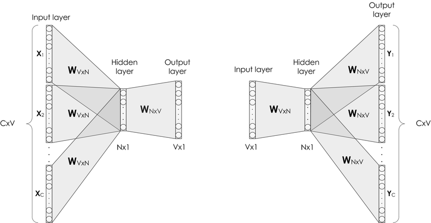
The same way word embeddings improved language modeling in many NLP tasks, items embeddings improved recommendation systems by applying the same concept though.
I read Ramzi Karam Blog post about how this technique is used on Anghami the leading music platform in MENA with more than 700 million users.
Types and Taxonomy of Recommendation Systems
- Items Popularity Based Models
- Collaborative Filtering Based Models
- Demographic Based Models
- Content Based Models
- Utility-based recommendation system
- Knowledge-based recommendation system
- Hybrid-recommendation system
- In this post i will be discuss the main characteristics of the first approach (Items
- Popularity Based Models) and later in others separate parts i will be talking about each one individually.
EDA and Features Engineering

EDA
The Full MovieLens data set consisting of 26 million ratings and 750,000 tag applications from 270,000 users on all the 45,000 movies in this data-set that we are going to use for our application. can be accessed here
## importing dependencies
import ast
import pandas as pd
import numpy as np
from ast import literal_eval
import matplotlib.pyplot as plt
plt.style.use('ggplot')
%matplotlib inline
Let’s load the MoviesLens data set
## load data
movies = pd.read_csv('./data/movies_metadata_edited.csv')
movies_subset = pd.read_csv('./data/links_small.csv')
ratings = pd.read_csv('./data/ratings_small.csv')
## drop NaN values and invalid ids
movies_subset = movies_subset.dropna().copy()
drop_idx = movies[movies.id.str.contains('-')].index.values.tolist()
movies = movies.drop(drop_idx)

## type mismatch issue
movies.id = movies.id.apply(int)
movies_subset['tmdbId'] = movies_subset['tmdbId'].apply(int)
It seems our data is a little bit large (45000 records) and may not fit into our memory, So we are going to chunk it a little bit:
## subset the data-set according to movies_subset table
print('We have {} rows before chunking'.format(len(movies)))

## chunck
movies = movies[movies.id.apply(int).isin(movies_subset.tmdbId.values.tolist())]

print('We have {} rows after chunking'.format(len(movies)))
We have 45463 rows before chunking
We have 9099 rows after chunking
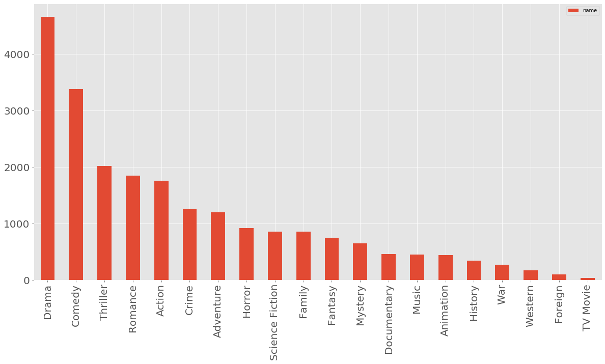
Now let’s see how many genres we have
## table for movies_genres relation
movies_to_genres = pd.DataFrame()

## function to relate movies with genres
def _movies_to_genres_map(row):
    records = literal_eval(row.genres)
    for rec in records:
        rec['movie_id'] = row.id
    return records

## record values to list of lists
genres_vals = movies.apply(_movies_to_genres_map, axis=1).values.tolist()

## flatten then construct new DataFrame
genres_vals = [y for x in genres_vals for y in x]
movies_to_genres = pd.DataFrame.from_dict(genres_vals)

## count each genre then plot bar plot
genres_counts = movies_to_genres.name.value_counts()
pd.DataFrame(genres_counts).plot.bar()

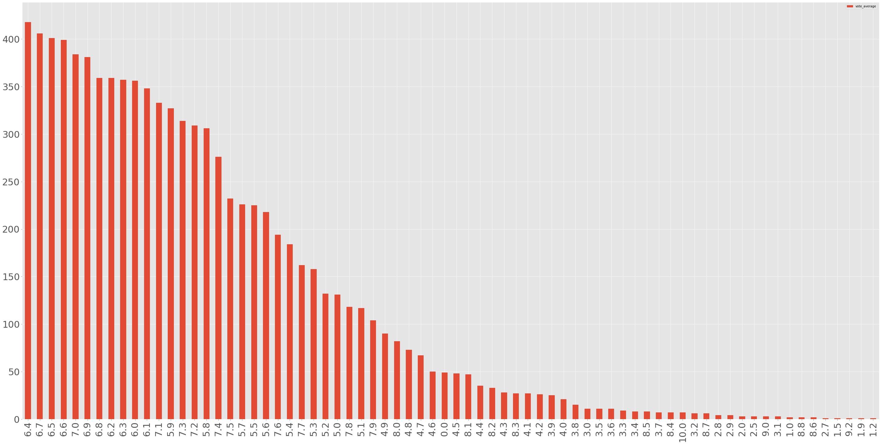
OK, then what is the most common rate

### pick ratings with only existing movieId in movies table
ratings = ratings[ratings.movieId.isin(movies.id)]
ratings.head(15)
OK, then what is the most common rate
userId	movieId	rating	timestamp
1	1371	2.5	1260759135
1	1405	1.0	1260759203
1	2105	4.0	1260759139
1	2193	2.0	1260759198
1	2294	2.0	1260759108
2	62	3.0	835355749
2	110	4.0	835355532
2	144	3.0	835356016
2	150	5.0	835355395
2	153	4.0	835355441
2	161	3.0	835355493
2	165	3.0	835355441
2	168	3.0	835355710
2	185	3.0	835355511
2	186	3.0	835355664
let’s take a look at the average rating of each movie. To do so, we can group the data set by the movieId & title of the movie and then calculate the mean of the rating for each movie
pd.merge(ratings, movies, on='movieId')[['userId', 'movieId', 'rating', 'title', 'vote_average', 'vote_count']]\
    .groupby(['movieId', 'title'])\
            .rating.mean()\
            .head(25)
movieId  title
2        Ariel                                                     3.401869
5        Four Rooms                                                3.267857
6        Judgment Night                                            3.884615
11       Star Wars                                                 3.689024
12       Finding Nemo                                              2.861111
13       Forrest Gump                                              3.937500
14       American Beauty                                           3.451613
15       Citizen Kane                                              2.318182
16       Dancer in the Dark                                        3.948864
18       The Fifth Element                                         3.288462
19       Metropolis                                                2.597826
20       My Life Without Me                                        2.538462
21       The Endless Summer                                        3.536842
22       Pirates of the Caribbean: The Curse of the Black Pearl    3.355263
24       Kill Bill: Vol. 1                                         3.044118
25       Jarhead                                                   3.742574
26       Walk on Water                                             4.100000
28       Apocalypse Now                                            4.083333
35       The Simpsons Movie                                        3.545455
38       Eternal Sunshine of the Spotless Mind                     2.000000
55       Amores perros                                             3.333333
58       Pirates of the Caribbean: Dead Man's Chest                4.000000
59       A History of Violence                                     4.000000
62       2001: A Space Odyssey                                     3.689655
63       Twelve Monkeys                                            2.833333
Name: rating, dtype: float64
## display the highest rates in deascending order
pd.merge(ratings, movies, on='movieId')[['userId', 'movieId', 'rating', 'title', 'vote_average', 'vote_count']]\
    .groupby(['movieId', 'title'])\
            .rating.mean().sort_values(ascending=False)\
            .head(25)
movieId  title
1771     Captain America: The First Avenger       5.0
309      The Celebration                          5.0
872      Singin' in the Rain                      5.0
2284     Mr. Magorium's Wonder Emporium           5.0
876      Frank Herbert's Dune                     5.0
103731   Mud                                      5.0
3021     1408                                     5.0
2981     The Lost World                           5.0
764      The Evil Dead                            5.0
759      Gentlemen Prefer Blondes                 5.0
1933     The Others                               5.0
26578    The Falcon and the Snowman               5.0
26422    The Pillow Book                          5.0
702      A Streetcar Named Desire                 5.0
2897     Around the World in Eighty Days          5.0
1563     Sunless                                  5.0
3580     Changeling                               5.0
4442     The Brothers Grimm                       5.0
301      Rio Bravo                                5.0
1450     Blood: The Last Vampire                  5.0
1428     Once Upon a Time in Mexico               5.0
4584     Sense and Sensibility                    5.0
8699     Anchorman: The Legend of Ron Burgundy    5.0
8675     Orgazmo                                  5.0
2636     The Specialist                           5.0
Name: rating, dtype: float64
let’s take a look at the number of users and the rating of each movie. A movie may be rated high by single user so it will appear at the top regardless of the number of users. In this case we may also use number of users that rated the same movie.
ratings_mean_user_counts = pd.DataFrame(
    pd.merge(ratings, movies, on='movieId')[['userId', 'movieId', 'rating', 'title', 'vote_average', 'vote_count']]\
        .groupby(['movieId', 'title']).rating.mean())

ratings_mean_user_counts['users_count'] = pd.merge(ratings, movies, on='movieId')[['userId', 'movieId', 'rating', 'title', 'vote_average', 'vote_count']]\
        .groupby(['movieId', 'title']).rating.count()

ratings_mean_user_counts.head(25)


ratings_mean_user_counts.rating.plot.hist(bins=50, figsize=(15, 10), grid=True, edgecolor='black', linewidth=1.2).set_axisbelow(True)
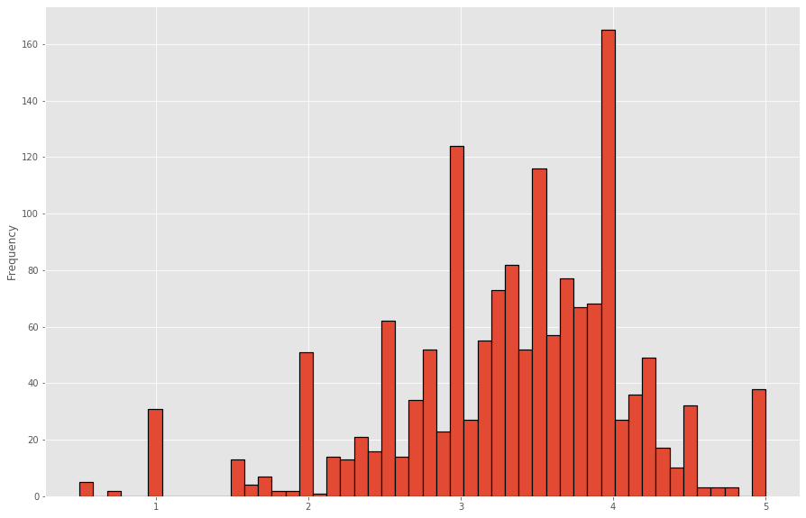
Most users rate movies with Integer Number according to the histogram
ratings_mean_user_counts.users_count.plot.hist(bins=50, figsize=(15, 10), edgecolor='black', linewidth=1.2)
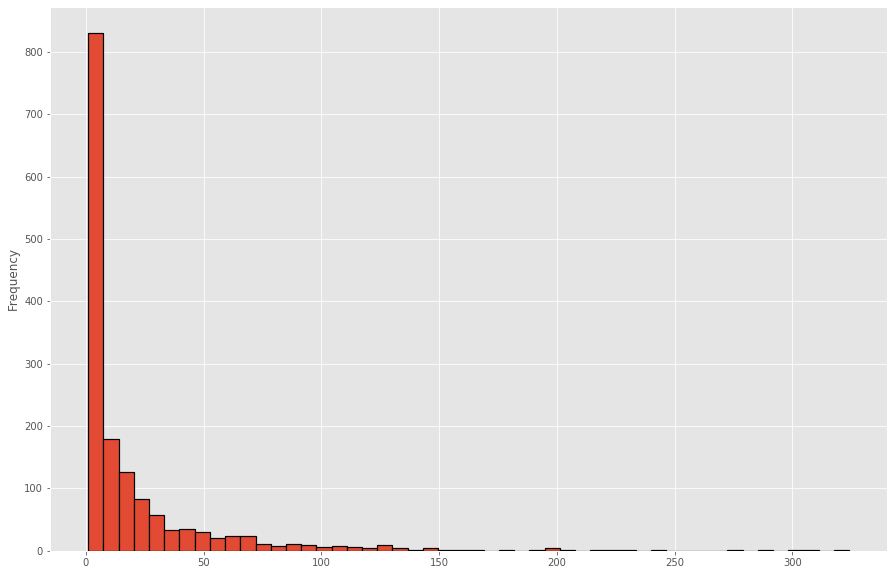
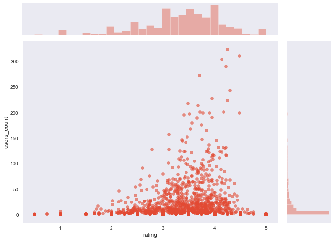
Normally, movies with a higher number of ratings usually have a high average rating as well since a good movie is normally well-known and a well-known movie is watched by a large number of users
pretty cool !
lets elaborate it visually:
import seaborn as snssns.set_style('dark')
sns.jointplot(x='rating', y='users_count', data=ratings_mean_user_counts, alpha=0.6).fig.set_size_inches(10,7)
Features Engineering
In this post we will focus on the simplest form of generating features vector to be used for every user and every item on our database.
Items Users Ranking Matrix
# User Items Ranking Matrix
# Construct Pivot Table that map between usersId and movieId this table is a Matrix # after all in which every row is user and columns is the movies he bought or rated.

## lets create Pivot table using pandas to relate usser_id and movie_id in Single Matrix
columns = ['userId', 'movieId', 'rating', 'title', 'vote_average', 'vote_count', 'poster_url']

movies_users_rates = pd.merge(ratings, movies, on='movieId')[columns]\
        .pivot_table(index='userId', columns='movieId', values='rating')

movies_users_rates.head(30)

Another One !
## lets create Pivot table using pandas to relate usser_id and movie_id in Single Matrix
columns = ['userId', 'movieId', 'rating', 'title', 'vote_average', 'vote_count', 'poster_url']
users_movies_rates = pd.merge(ratings, movies, on='movieId')[columns]\
        .pivot_table(index='movieId', columns='userId', values='rating')
users_movies_rates.head(30)
We could use either of them to make predictions according to the selected movie or the selected user.
## it's cool that panadas support most of numpy utilities

# rotate to transpose the matirx
users_movies_rates = movies_users_rates.T
Notice You may notice too many NaN in the matrix, however, this is not a problem given the fact that not every user will rate every movie in the database so, i guess it makes sense.
Assume we are using the first Matrix which is a mapping between ranked movies and users, each row represent movies ranking vector. A movie is clicked to be bought or watched or whatever, then what we need to do is measure the similarity between this movie vector and all movies samples in our database, then recommend the most similar one.
Cosine Similarity We could use cosine similarity to measure how items is similar, or how users may be related in movies taste.
If user is watching Terminator what is the most similar movie that can be recommended or this user MAY ALSO LIKE.
Cosine Similarity
Now we can recommend similar movies by measuring similarity between this movie and all other movies samples in our database, the smaller the angle between vectors the more similar the users or the items according to what we are measuring.
import numpy as np

def cosine_similarity(a, b):
    """
    Calculate the cosine angle between two vectors according to the dot product definition
    """
    return np.dot(a, b) / np.linalg.norm(a)*np.linalg.norm(b)


from sklearn.metrics.pairwise import cosine_similarity

# however it is available by just calling

# between two vectors
cosine_similarity(a, b)

# between all samples of vector
cosine_similarity(a)

X = movies_users_rates
Y = movies_users_rates[movie_id].values.reshape(-1, 1)
cosine_sim = cosine_similarity(X.T, Y.T)
A movie may be rated high by single user so it will appear at the top regardless of the number of users. In this case number of users attribute should be taken into consideration.
Normally, movies with a higher number of ratings usually have a high average rating as well since a good movie is normally well-known and a well-known movie is watched by a large number of users. check the above graph.
cosine_sim_df = pd.DataFrame(cosine_sim, columns=['cosine_sim'], index=movies_users_rates.T.index)\
.reset_index('movieId').head(500)
cosine_sim_df['title'] = movies[movies.movieId.isin(cosine_sim_df.movieId)].copy()\
.sort_values('movieId').title.values
cosine_sim_df['poster_url'] = movies[movies.movieId.isin(cosine_sim_df.movieId)].copy()\
.sort_values('movieId').poster_url.values
cosine_sim_df['rate'] = movies[movies.movieId.isin(cosine_sim_df.movieId)].copy()\
.sort_values('movieId').vote_average.values
cosine_sim_df['users_count'] = ratings_mean_user_counts.head(500).users_count.values
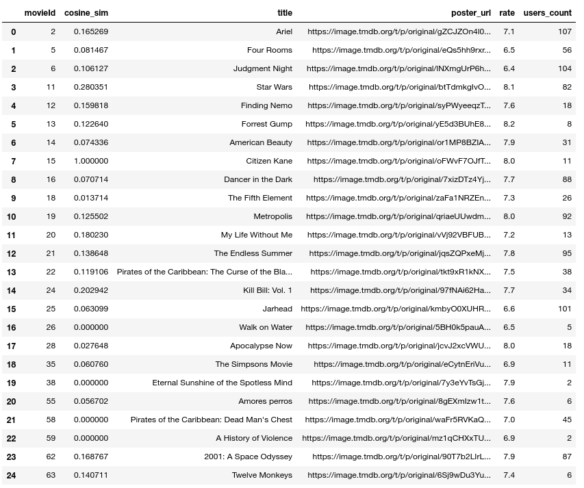
cosine_sim_df.head(25)
Now lets see the top k items
## Now lets see the top k items
top_k = cosine_sim_df.query('cosine_sim > 0.3 & users_count > 10').\
                            sort_values('cosine_sim', ascending=False).head(15)
top_k

Pearson Correlation Recommender
Correlation Coefficient is measure of how closely two variables move in relation to one another. The range of correlation values is between (-1, 1).
There are several types of correlation coefficients but, Pearson correlation is the one most commonly used in statistics. This measures the strength and direction of a linear relationship between two variables.
A correlation approaches value = 1.0 If
Xgoes up by one unit thenYwill also goes up by one unit
A correlation approaches value = 0.0
XandYis not co-related by any means
A correlation approaches value = -1.0 If
Xgoes up by one unit thenYwill goes down by one unit
Notice: This type of Correlation can fit only on linear relationship between two variables.
How this really works?
We can use relation between movies and users ranking to find recommendations and suggest it to similar users and that can be achieved by using correlation coefficient similarity.
Enough Blablah and show me how?
The Features Vector may look like the following image, it is user ratings matrix that can be used to correlate users together according to their ratings of the items whether it is products, songs, movies …. etc.
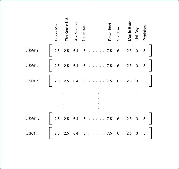
It seems the algorithm calculates how much two users are correlated. If their trends are identical (like similar movies) then they go up and down together Correlation=1.0 on the other hand if the Correlation=-1.0 then what one like the other dislike.
Let’s get back to some coding
print('Top 15 Movies similar to this:')

pearson_sim = movies_users_rates.corrwith(movies_users_rates[movie_id])

print(pearson_sim.sort_values(ascending=False).head(15))

Movie Id 507
Top 15 Movies similar to this:
movieId
507     1.000000
2749    0.480773
1791    0.471858
2577    0.467459
2757    0.463661
425     0.450372
5680    0.443091
3036    0.433864
695     0.430148
3526    0.429513
1124    0.420069
1366    0.418086
2267    0.414850
1396    0.412026
1266    0.404898
dtype: float64
pearson_sim_df = pd.DataFrame(pearson_sim, columns=['pearson_sim'])\
                        .reset_index('movieId').head(500)

pearson_sim_df['title'] = movies[movies.movieId.isin(pearson_sim_df.movieId)].copy()\
                        .sort_values('movieId').title.values

pearson_sim_df['poster_url'] = movies[movies.movieId.isin(pearson_sim_df.movieId)].copy()\
                        .sort_values('movieId').poster_url.values

pearson_sim_df['rate'] = movies[movies.movieId.isin(pearson_sim_df.movieId)].copy()\
                        .sort_values('movieId').vote_average.values

pearson_sim_df['users_count'] = ratings_mean_user_counts.head(500).users_count.values

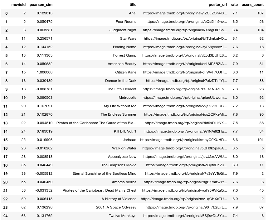
pearson_sim_df.head(25)

## Now lets see the top k items
top_k = pearson_sim_df.query('pearson_sim > 0.3 & users_count > 10')\
                .sort_values('pearson_sim', ascending=False).head(15)

top_k

Remark
it seems that this way of representing data and constructing matrix to feed into recommender systems algorithm is simple, however, it has several defects. one of those effects is how the information terms may not overlap (Sparse Vector) due to many zeros in the matrix which may lead to loss of context of the information. this problem even though may be partially solved using one of the available dimensionality reduction techniques such as SVD, PCA and T-SNE.
Live Demo Available Here !
References