Multi Handwritten Digits Recognition In Nutshell
RNN CNN hybrid models for identifying sequence of arbitrary digits in single image. Exploring different models architectures related to sequence classification and Multi-label images classification.
I participated in udacity deep learning [https://classroom.udacity.com/courses/ud730] online course long time ago and learned about modern neural networks and various architectures of them like convolution neural network (CNN) and recurrent neural network (RNN).
The final project of the course was to build a live camera app that can read and decode sequence of digits from natural images and prints the numbers it sees in real time.
I didn’t know where to start from even i participated in the course and understood the basic concepts, but really practicing and implementing is different from just finishing the course. I had many thoughts in my mind and really wanted to implement most of them. In this Post i am going to list and illustrate how i build different models architectures to solve such a problem.
Objective | Problem Definition
- We have Input image contains sequence of digits [0 - 9] and our goal is to recognize this arbitrary sequences.
- this problem can be considered as Multi-label Image Classification problem modeling since we have sequence of digits in a single image and sequence of output label for each digit.
- If you don’t know the difference between Multi-label and Multi-Class classification problem i recommend to read it from here ! [https://gombru.github.io/2018/05/23/cross_entropy_loss/]
- Constraints: the sequence of digits must be of limited size. The neural network will not recognize (more than N digits).
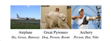
Images of multi label from this paper
Dataset
The main thing you’ll want to read about next is probably: what are the available datasets that we are going to use. MNIST [http://yann.lecun.com/exdb/mnist/] is like the “Hello World” of machine learning. Its a database of handwritten digits (0-9), with which you can try out a few machine learning algorithms. Many machine learning libraries like scikit-learn or keras in python already provide easy access to the MNIST dataset.
If you want to go wilder then you can experiment with The Street View House Numbers (SVHN) [http://ufldl.stanford.edu/housenumbers/] dataset which is is a dataset of about 200k street numbers along with bounding boxes and labels for individual digits, giving about 600k digits total. SVHN is obtained from house numbers in Google Street View images.
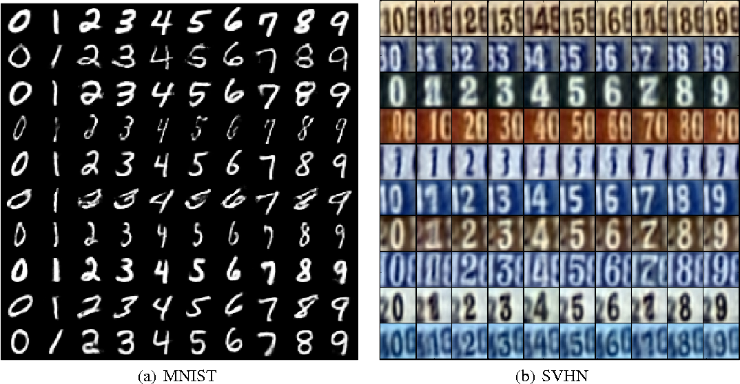
SVHN and MNIST looks like !But, Mnist exists only for individual digits how to construct sequence of digits, and the answer is pretty simple just stack them horizontally or vertically. and for sake of augmentation and variety of the training examples you can do the following:
- rotate each of the digits with random degree (maximum 45°) so no ambiguity occures between (6 and 9) digits.
- shift the digits randomly but consider intersection between them (make sure they are not intersected).
- the more permutation between the digits in sequence the better training examples will be to overcome over-fitting (High Variance) problem.
The dataset code generator available on github. Convolutional Neural Networks (CNN) My First Approach was to use convolutional neural network (CNN), of course CNN achieved state of the art solution in many computer vision and natural language processing tasks. CNN is capable of capturing complex features from images by preserving spatial information which is applicable by learnable kernels (filters) on the original input images. This what makes CNN superior at capturing complex patterns like (Edges, Blurred Areas, Specific Shapes and Objects…etc.
How is that and what does spatial term mean ? In Regular Neural Networks (NN) You Simply Flatten the input image then feed it directly to the neurons so every pixel of the image would be connected to next hidden neurons in the network and that would be of high complexity when it comes to computation. Besides ignoring the spatial structure of the image. That what makes CNN awesome in vision tasks as it keeps spatial information in their filters and Sampling image to extract features from its local receptive field.
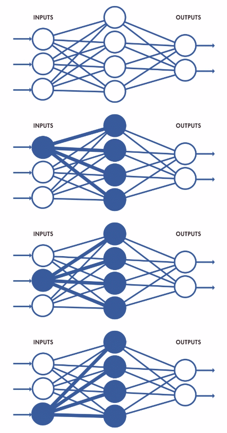
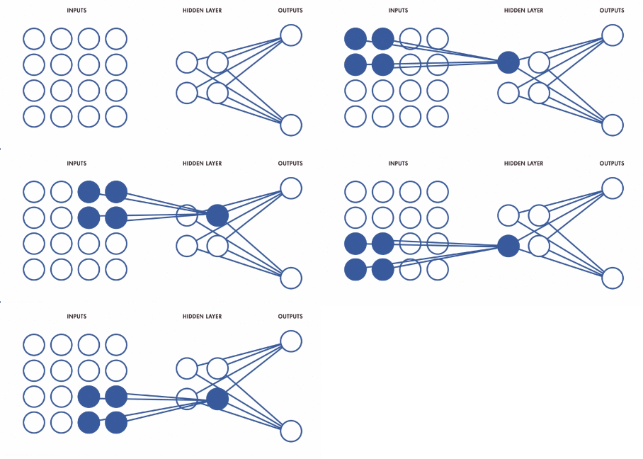
regular neural network and convolution sampling Now let’s see how our CNN looks like to recognize sequence of digits:
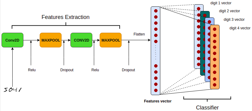
Now it is time for some coding, for sake of simplicity and life is too short use Keras functional API which uses tensorflow backend, The first thing i am going to do is import the dependencies then define our model in a sequential flow:
## dependencies import
import cv2
import numpy as np
import keras as K
import keras.layers as L
import keras.models as M
from keras.datasets import mnist
from time import time
## CNN Sequential model from keras Functional API
cnn_model = M.Sequential()
cnn_model.add(L.InputLayer((h, w, d)))
cnn_model.add(L.Conv2D(filters=16, kernel_size=(3, 3), strides=1, padding='same', activation='relu'))
cnn_model.add(L.MaxPool2D(pool_size=(2, 2)))
cnn_model.add(L.Dropout(0.2))
cnn_model.add(L.Conv2D(filters=32, kernel_size=(3, 3), strides=1, padding='same', activation='relu'))
cnn_model.add(L.MaxPool2D(pool_size=(2, 2)))
cnn_model.add(L.Dropout(0.2))
cnn_model.add(L.Flatten())
cnn_model.add(L.Dense(128))
cnn_model.add(L.Dropout(0.5))

inputs = L.Input(shape=(h, w, d))
outputs = [L.Dense(10, activation='softmax')(cnn_model.output) for _ in range(4)]

dcnn_model = K.Model(cnn_model.input, outputs)
dcnn_model.compile(loss='categorical_crossentropy', optimizer='adam', metrics=['categorical_accuracy'])
If you are new to machine learning you may be asking what is the term “ categorical_crossentropy” means and why “softmax” is used as an activation function ? Here is the deal ! When you work with machine learning problem you have to make sure of your data structure (input/output) and how it should be look and ask yourself does it make sense or not in order to define your correct objective (loss function).
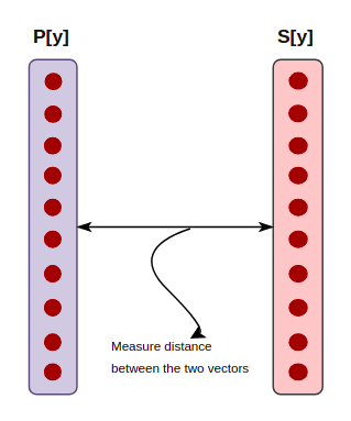
Crossentropy Loss
Cross Entropy loss is used to measure how well the classifier performs, it measures the distance between the probabilities distribution from the feed forward operations (Scores calculation) in the neural network and the ground truth labels. In this case let’s denote S[y] as the ground truth and P[y] as the probability distribution from activating the logits/scores of the final hidden layer. If you have been reading deep learning papers before which is highly recommended to increase your knowledge about state of the art solutions in many tasks you may find many versions of Cross-entropy Loss which is listed below with the difference and the objective for each. For more details about the available losses in keras read this [https://keras.io/losses/]:
- Categorical Cross-entropy

Categorical one hot encoding
dcnn_model.compile(loss='categorical_crossentropy', optimizer='adam', metrics=['categorical_accuracy'])
- Binary Cross-entropy

Binary one hot encoding
dcnn_model.compile(loss='binary_crossentropy', optimizer='adam', metrics=['binary_accuracy'])
- Sparse Categorical Cross-entropy

dcnn_model.compile(loss='sparse_categorical_crossentropy', optimizer='adam', metrics=['sparse_categorical_accuracy'])
Here is the thing !
keep in mind this, Defining your loss function is very important when you are dealing with classification problems, it depends on how your output looks like and how to encode a wild data that you may find and don’t expect to find data and how to encode a wild data that you may find and don’t expect to find data with the exact structure in your mind.
Now the results looks like:
Train on 20000 samples, validate on 5000 samples
Epoch 1/6
20000/20000 [==============================] - 342s 17ms/step - loss: 2.5658 - dense_2_loss: 0.6757 - dense_3_loss: 0.6335 - dense_4_loss: 0.6382 - dense_5_loss: 0.6184 - dense_2_acc: 0.8915 - dense_3_acc: 0.8960 - dense_4_acc: 0.8931 - dense_5_acc: 0.8976 - val_loss: 0.5233 - val_dense_2_loss: 0.1437 - val_dense_3_loss: 0.1170 - val_dense_4_loss: 0.1455 - val_dense_5_loss: 0.1172 - val_dense_2_acc: 0.9477 - val_dense_3_acc: 0.9592 - val_dense_4_acc: 0.9471 - val_dense_5_acc: 0.9573
Epoch 2/6
20000/20000 [==============================] - 342s 17ms/step - loss: 0.5981 - dense_2_loss: 0.1670 - dense_3_loss: 0.1331 - dense_4_loss: 0.1655 - dense_5_loss: 0.1324 - dense_2_acc: 0.9384 - dense_3_acc: 0.9496 - dense_4_acc: 0.9385 - dense_5_acc: 0.9503 - val_loss: 0.2334 - val_dense_2_loss: 0.0662 - val_dense_3_loss: 0.0473 - val_dense_4_loss: 0.0717 - val_dense_5_loss: 0.0481 - val_dense_2_acc: 0.9780 - val_dense_3_acc: 0.9859 - val_dense_4_acc: 0.9754 - val_dense_5_acc: 0.9856
Epoch 3/6
20000/20000 [==============================] - 341s 17ms/step - loss: 0.4173 - dense_2_loss: 0.1169 - dense_3_loss: 0.0902 - dense_4_loss: 0.1220 - dense_5_loss: 0.0883 - dense_2_acc: 0.9570 - dense_3_acc: 0.9665 - dense_4_acc: 0.9548 - dense_5_acc: 0.9670 - val_loss: 0.1346 - val_dense_2_loss: 0.0446 - val_dense_3_loss: 0.0236 - val_dense_4_loss: 0.0431 - val_dense_5_loss: 0.0232 - val_dense_2_acc: 0.9856 - val_dense_3_acc: 0.9938 - val_dense_4_acc: 0.9867 - val_dense_5_acc: 0.9937
Epoch 4/6
20000/20000 [==============================] - 342s 17ms/step - loss: 0.3193 - dense_2_loss: 0.0954 - dense_3_loss: 0.0664 - dense_4_loss: 0.0921 - dense_5_loss: 0.0653 - dense_2_acc: 0.9650 - dense_3_acc: 0.9756 - dense_4_acc: 0.9658 - dense_5_acc: 0.9757 - val_loss: 0.0863 - val_dense_2_loss: 0.0283 - val_dense_3_loss: 0.0154 - val_dense_4_loss: 0.0287 - val_dense_5_loss: 0.0140 - val_dense_2_acc: 0.9913 - val_dense_3_acc: 0.9964 - val_dense_4_acc: 0.9913 - val_dense_5_acc: 0.9970
Epoch 5/6
20000/20000 [==============================] - 342s 17ms/step - loss: 0.2582 - dense_2_loss: 0.0762 - dense_3_loss: 0.0533 - dense_4_loss: 0.0782 - dense_5_loss: 0.0505 - dense_2_acc: 0.9719 - dense_3_acc: 0.9803 - dense_4_acc: 0.9712 - dense_5_acc: 0.9812 - val_loss: 0.0563 - val_dense_2_loss: 0.0186 - val_dense_3_loss: 0.0091 - val_dense_4_loss: 0.0196 - val_dense_5_loss: 0.0090 - val_dense_2_acc: 0.9947 - val_dense_3_acc: 0.9980 - val_dense_4_acc: 0.9949 - val_dense_5_acc: 0.9980
Epoch 6/6
20000/20000 [==============================] - 344s 17ms/step - loss: 0.2174 - dense_2_loss: 0.0650 - dense_3_loss: 0.0436 - dense_4_loss: 0.0663 - dense_5_loss: 0.0425 - dense_2_acc: 0.9763 - dense_3_acc: 0.9840 - dense_4_acc: 0.9755 - dense_5_acc: 0.9840 - val_loss: 0.0342 - val_dense_2_loss: 0.0123 - val_dense_3_loss: 0.0048 - val_dense_4_loss: 0.0126 - val_dense_5_loss: 0.0045 - val_dense_2_acc: 0.9967 - val_dense_3_acc: 0.9991 - val_dense_4_acc: 0.9970 - val_dense_5_acc: 0.9992
Recurrent Neural Networks (RNN)
So far we discussed how convolutional neural network (CNN) operates and we built a model that can extract complex information from images by keeping the spatial dimension. In this section i am going to explain how to use Recurrent Neural Network (RNN) to solve the same problem.
Basically Recurrent Neural Network (RNN) are designed to allow deep networks to handle sequence of data where the sequence of data matters like (speech, video, text).
If you want to read more about the internal work of RNN, no one illustrate it better than Christopher Olah [http://colah.github.io/posts/2015-08-Understanding-LSTMs/].
Now what about our problem, how to train recurrent neural network (RNN) to read sequence of pixels in an image and decode it to sequence of predictions based on this features. In the following diagrams i made it as simple as possible to get intuition about the mechanism of recurrent neural network (RNN) and how it operates internally. We feed each row of the training samples in sequential manner so each row is processed in a single step of the network through (feed forward) pass operation.
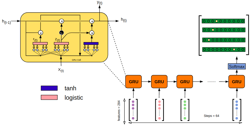
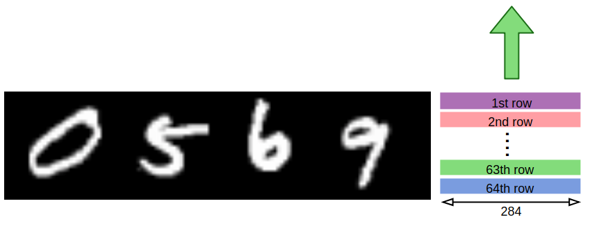
Now time for some coding to get better overview if you don’t catch up yet.
import keras as K
import keras.layers as L
import keras.models as M

n_steps = h ## rows steps
n_features = w ## columns features

## GRU Cell with 40 hidden units
gru = L.GRU(units=40)

## Fully connected output layer
dense = L.Dense(10, activation="softmax")

reshape = L.Reshape((4, 10))

inp = L.Input((n_steps, n_features))

out = gru(inp)
out = reshape(out)
out = dense(out)

model = M.Model(inp, out)

model.summary()
_________________________________________________________________
Layer (type)                 Output Shape              Param #
=================================================================
input_1 (InputLayer)         (None, 64, 208)           0
_________________________________________________________________
gru_1 (GRU)                  (None, 40)                29880
_________________________________________________________________
reshape_1 (Reshape)          (None, 4, 10)             0
_________________________________________________________________
dense_1 (Dense)              (None, 4, 10)             110
=================================================================
Total params: 29,990
Trainable params: 29,990
Non-trainable params: 0
_________________________________________________________________
model.compile(loss='categorical_crossentropy', optimizer=K.optimizers.adam(), metrics=['categorical_accuracy'])
Now time for training …
model_hist = model.fit(
    x=X_train, y=Y_train,
    epochs=100,
    batch_size=128,
    validation_data=(X_test, Y_test)
)
Epoch 95/100
15000/15000 [==============================] - 11s 755us/step - loss: 0.2711 - categorical_accuracy: 0.9150 - val_loss: 0.3019 - val_categorical_accuracy: 0.9030
Epoch 96/100
15000/15000 [==============================] - 11s 749us/step - loss: 0.2758 - categorical_accuracy: 0.9111 - val_loss: 0.2508 - val_categorical_accuracy: 0.9313
Epoch 97/100
15000/15000 [==============================] - 11s 748us/step - loss: 0.2289 - categorical_accuracy: 0.9351 - val_loss: 0.2312 - val_categorical_accuracy: 0.9363
Epoch 98/100
15000/15000 [==============================] - 11s 750us/step - loss: 0.2250 - categorical_accuracy: 0.9357 - val_loss: 0.2438 - val_categorical_accuracy: 0.9260
Epoch 99/100
15000/15000 [==============================] - 11s 747us/step - loss: 0.2242 - categorical_accuracy: 0.9362 - val_loss: 0.2870 - val_categorical_accuracy: 0.9070
Epoch 100/100
15000/15000 [==============================] - 11s 752us/step - loss: 0.2577 - categorical_accuracy: 0.9180 - val_loss: 0.2291 - val_categorical_accuracy: 0.9340
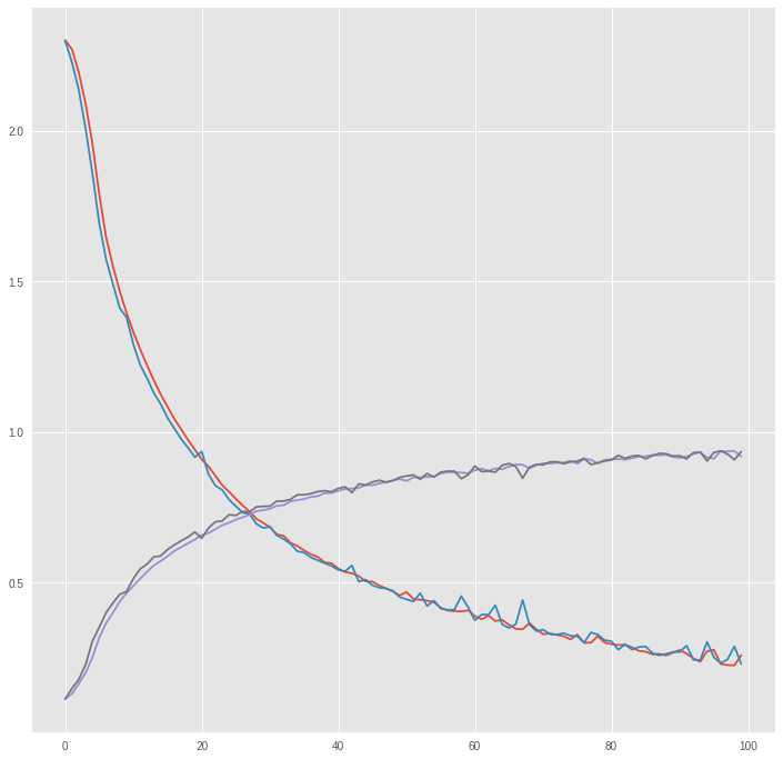
Let’s plot the result for inference and checking out over-fitting and the model performance
import matplotlib.pyplot as plt
plt.style.use("ggplot")
plt.figure(figsize=(12,12))
plt.plot(model_hist.history["loss"])
plt.plot(model_hist.history["val_loss"])
plt.plot(model_hist.history["categorical_accuracy"])
plt.plot(model_hist.history["val_categorical_accuracy"])
plt.show()
training and validation performance
